

Factor Graph Optimization for GNSS/INS Integration: A Comparison with the Extended Kalman Filter
NAVIGATION: Journal of the Institute of Navigation (2021)
Summary
Factor graph optimization recasts GNSS/INS integration as a sliding-window estimation problem rather than a one-epoch filtering problem.
Highlights
- Compares EKF and FGO for both loosely coupled and tightly coupled GNSS/INS integration.
- Uses an urban-canyon experiment in Hong Kong with low-cost GNSS, INS, fisheye imagery, and ground-truth reference equipment.
- Shows that sliding-window FGO can revisit historical states and reduce the impact of outliers and non-Gaussian GNSS errors.
Figures
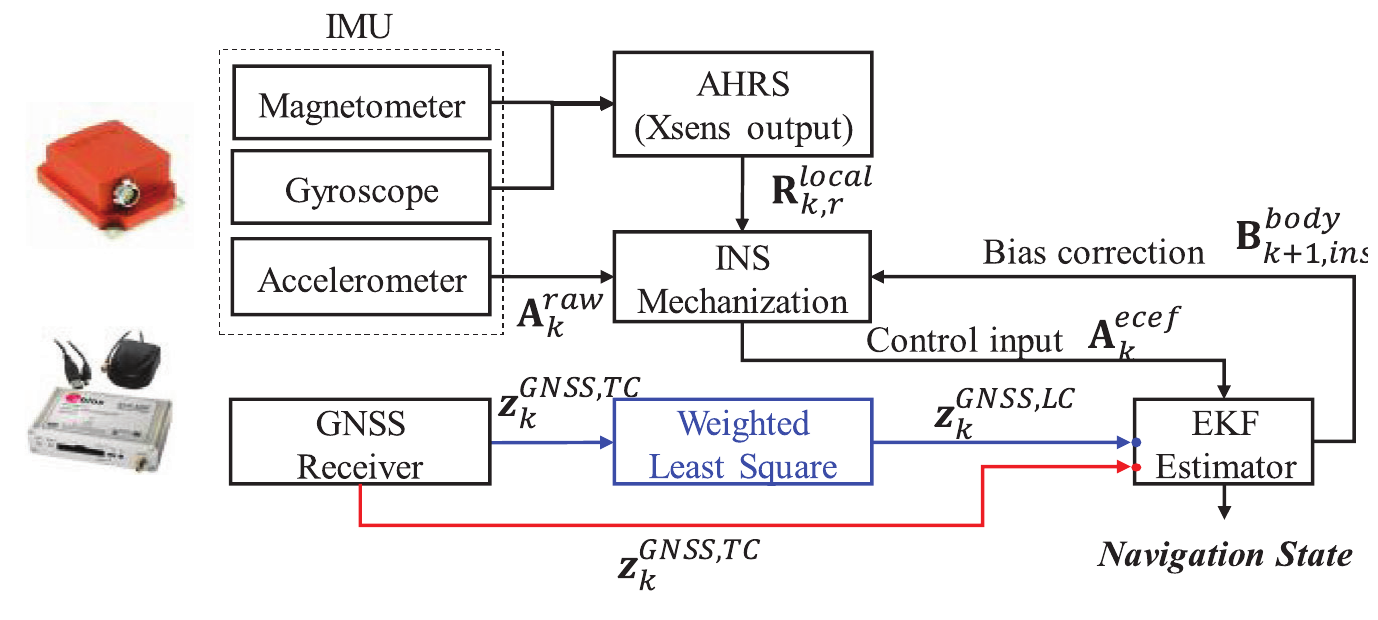
Before the factor graph model, the paper first establishes the EKF loosely coupled and tightly coupled baselines that the new formulation is compared against.
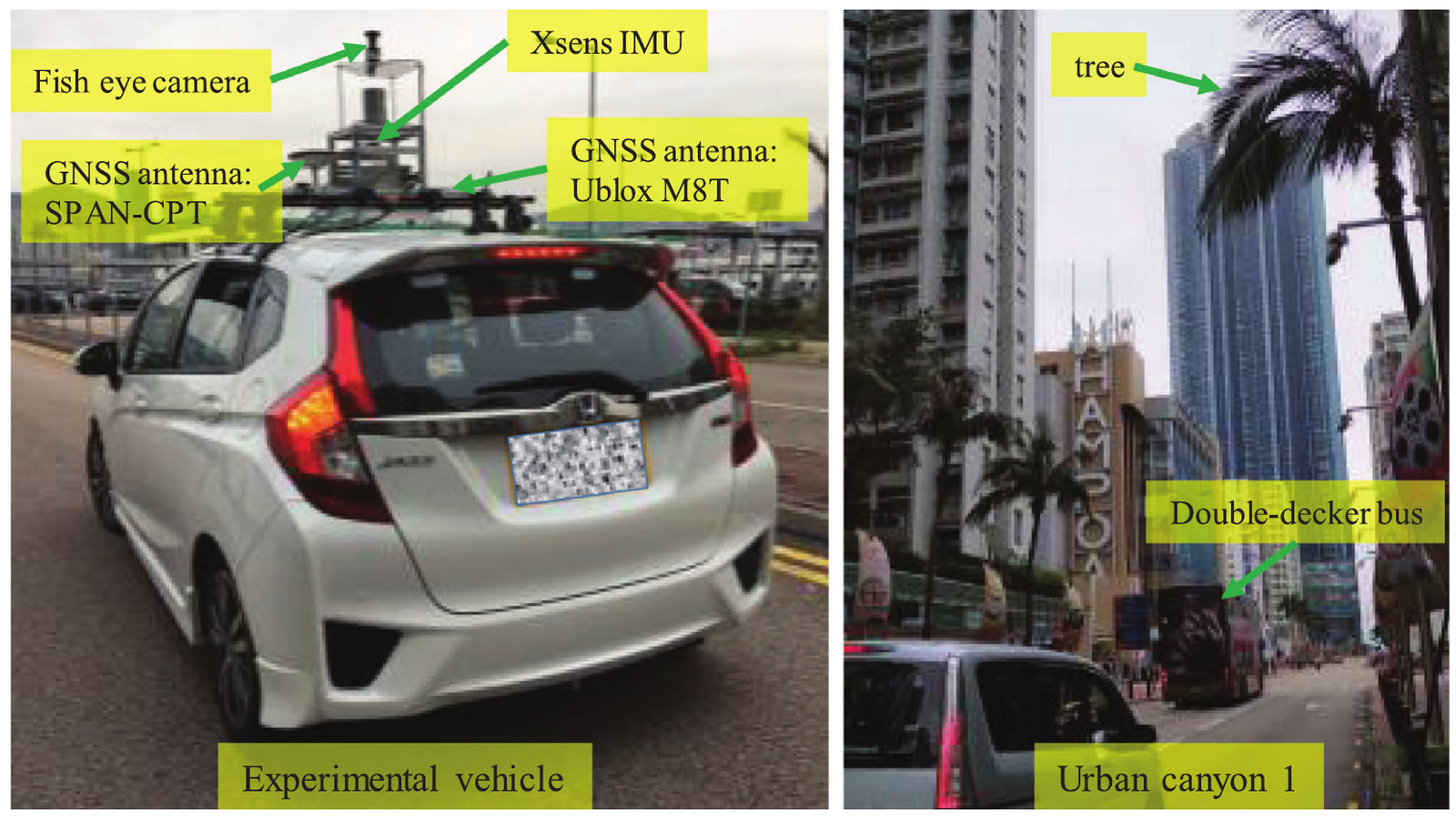
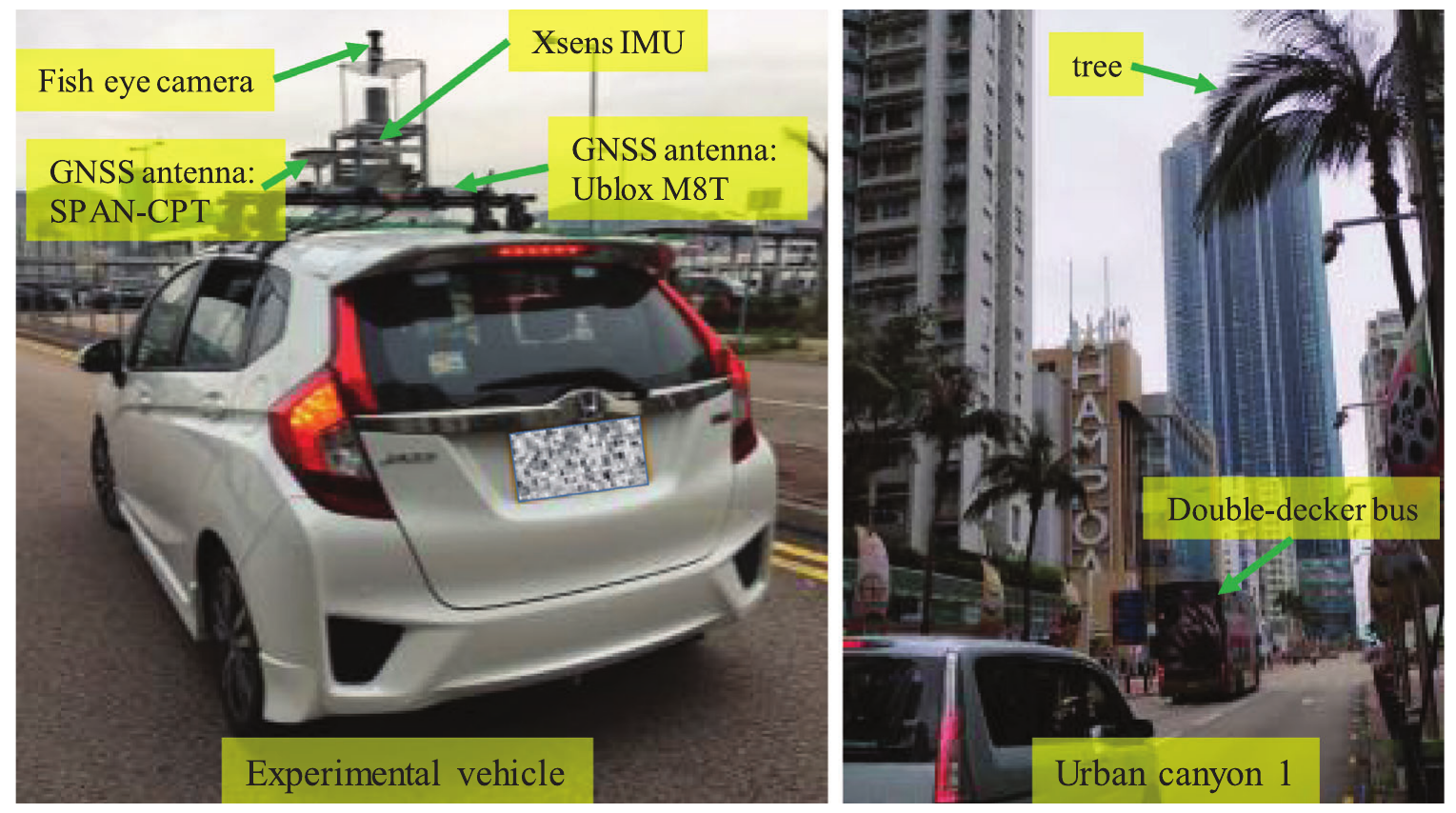
After defining the estimation structure, the paper moves to the Hong Kong vehicle setup and urban canyon route used for the EKF-versus-FGO comparison.
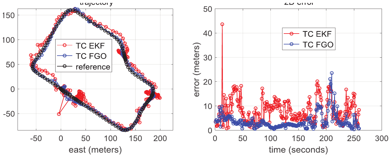
The first main result turns the method into trajectory evidence by comparing tightly coupled EKF and FGO against the reference path.
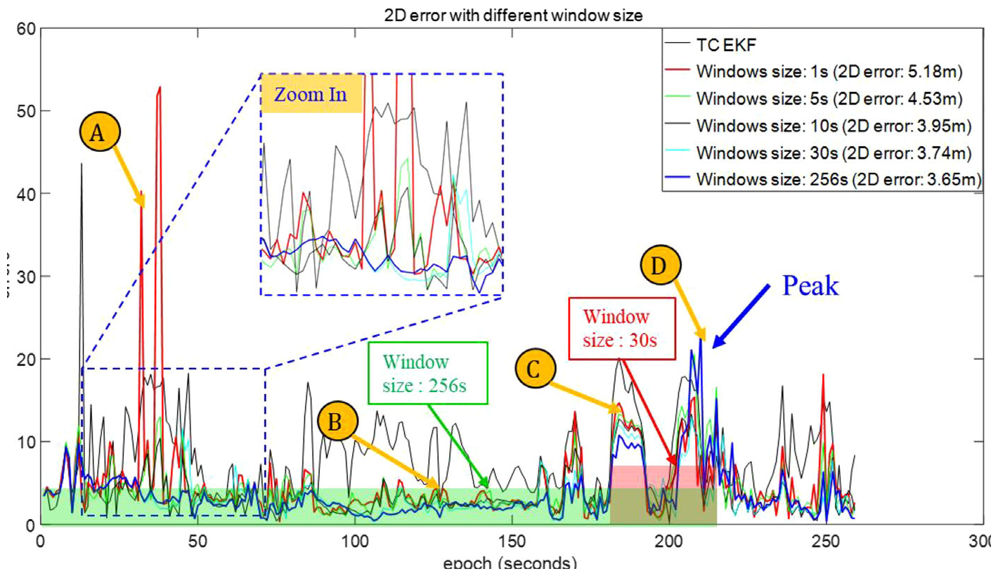
The window-size study explains why FGO performance depends on how much historical information is optimized together.
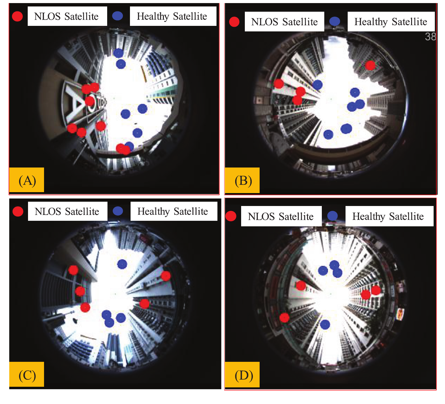
These sky-view epochs interpret the window-size result by showing the LOS/NLOS satellite conditions during difficult periods.
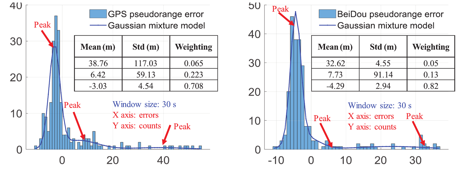
The pseudorange histograms connect the positioning behavior to non-Gaussian urban measurement noise.
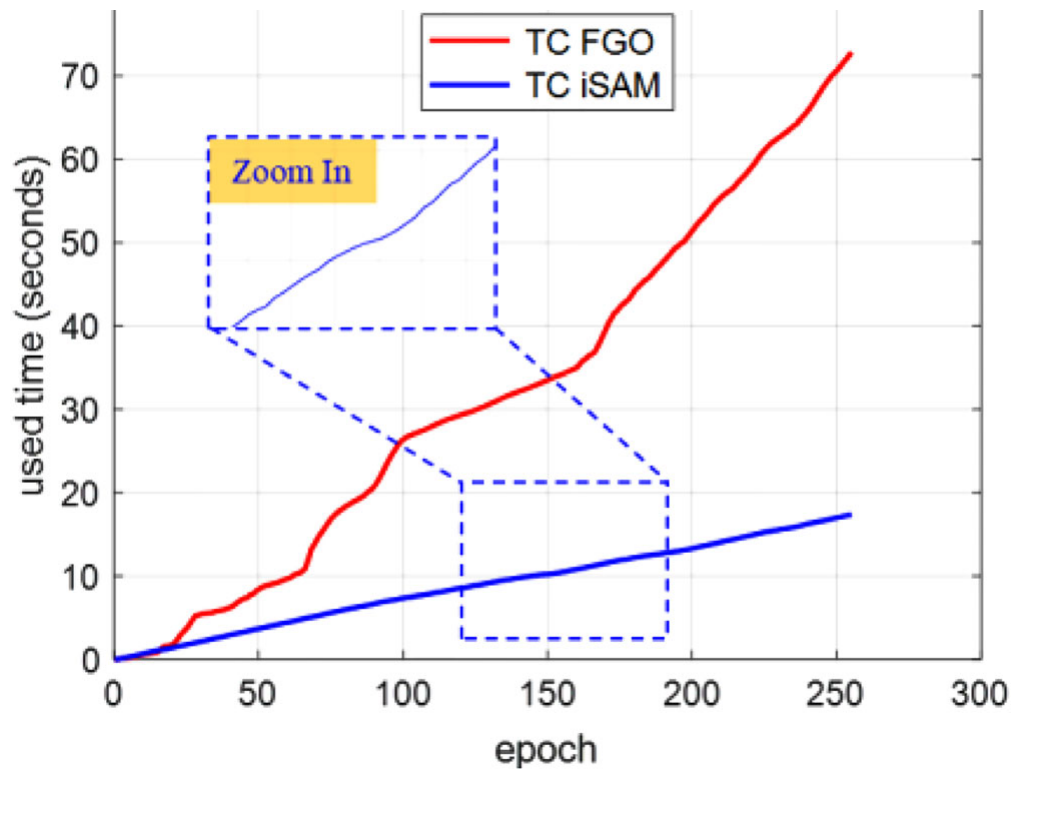
The final comparison checks the practical computation cost of solving the tightly coupled graph with FGO versus iSAM.
Key idea. Classical GNSS/INS integration uses an Extended Kalman Filter, which condenses all history into a single current state. This paper recasts the problem as factor graph optimization (FGO) — jointly optimizing a sliding window of states with re-linearization, so the estimator can revisit past epochs and handle outliers far more flexibly.
Impact. It became the reference comparison establishing why FGO outperforms filtering for navigation, and was named the 2024 Most-Cited Paper in NAVIGATION. The result reframed how the field approaches GNSS/INS fusion and underpins much of IPNL’s later integrity and multi-sensor work.